
Big Data Project: Yelp Rating Regression Predictor
Published:
Yelp Rating Regression Predictor
1 Introduction
When deciding where to eat, I’ll often use Yelp: a crowd-sourced review service where users can rate restaurants on a scale from 1 to 5 stars (5 being the best possible rating.) Considering that a restaurant’s success is highly correlated with its reputation, it can be useful to understand the underlying features that can affect its online perception.
In this project, I will use a Multiple Linear Regression model to investigate the features that most directly affect a restaurant’s Yelp rating and consequently use these features to predict Yelp ratings of hypothetical restaurants.
1.1 Goal:
- Demonstrate how a Multiple Linear Regression model can be used to predict a restaurant’s Yelp rating
1.2 Approach:
- Perform statistical analysis on a real Yelp dataset comprised of 6
jsonfiles.yelp_business.json: establishment data regarding location and attributes for all businesses in the datasetyelp_review.json: Yelp review metadata by businessyelp_user.json: user profile metadata by businessyelp_checkin.json: online checkin metadata by businessyelp_tip.json: tip metadata by businessyelp_photo.json: photo metadata by business
1.3 Imports
Import libraries and write settings here.
# Data manipulation
import pandas as pd
import numpy as np

# Options for pandas
pd.options.display.max_columns = 60
pd.options.display.max_rows = 500

# Machine Learning
from sklearn.model_selection import train_test_split
from sklearn.linear_model import LinearRegression

# Visualizations
%matplotlib inline
import matplotlib.pyplot as plt
2 Data Cleaning
2.1 Load the Data
First, let’s use Pandas to investigate the data in DataFrame form.
businesses = pd.read_json('yelp_business.json',lines=True)
reviews = pd.read_json('yelp_review.json',lines=True)
users = pd.read_json('yelp_user.json',lines=True)
checkins = pd.read_json('yelp_checkin.json',lines=True)
tips = pd.read_json('yelp_tip.json',lines=True)
photos = pd.read_json('yelp_photo.json',lines=True)
Let’s preview the first five rows of each DataFrame.
businesses.head()
| address | alcohol? | attributes | business_id | categories | city | good_for_kids | has_bike_parking | has_wifi | hours | is_open | latitude | longitude | name | neighborhood | postal_code | price_range | review_count | stars | state | take_reservations | takes_credit_cards | |
|---|---|---|---|---|---|---|---|---|---|---|---|---|---|---|---|---|---|---|---|---|---|---|
| 0 | 1314 44 Avenue NE | 0 | {'BikeParking': 'False', 'BusinessAcceptsCredi... | Apn5Q_b6Nz61Tq4XzPdf9A | Tours, Breweries, Pizza, Restaurants, Food, Ho... | Calgary | 1 | 0 | 0 | {'Monday': '8:30-17:0', 'Tuesday': '11:0-21:0'... | 1 | 51.091813 | -114.031675 | Minhas Micro Brewery | T2E 6L6 | 2 | 24 | 4.0 | AB | 1 | 1 | |
| 1 | 0 | {'Alcohol': 'none', 'BikeParking': 'False', 'B... | AjEbIBw6ZFfln7ePHha9PA | Chicken Wings, Burgers, Caterers, Street Vendo... | Henderson | 1 | 0 | 0 | {'Friday': '17:0-23:0', 'Saturday': '17:0-23:0... | 0 | 35.960734 | -114.939821 | CK'S BBQ & Catering | 89002 | 2 | 3 | 4.5 | NV | 0 | 1 | ||
| 2 | 1335 rue Beaubien E | 1 | {'Alcohol': 'beer_and_wine', 'Ambience': '{'ro... | O8S5hYJ1SMc8fA4QBtVujA | Breakfast & Brunch, Restaurants, French, Sandw... | Montréal | 1 | 1 | 1 | {'Monday': '10:0-22:0', 'Tuesday': '10:0-22:0'... | 0 | 45.540503 | -73.599300 | La Bastringue | Rosemont-La Petite-Patrie | H2G 1K7 | 2 | 5 | 4.0 | QC | 1 | 0 |
| 3 | 211 W Monroe St | 0 | None | bFzdJJ3wp3PZssNEsyU23g | Insurance, Financial Services | Phoenix | 0 | 0 | 0 | None | 1 | 33.449999 | -112.076979 | Geico Insurance | 85003 | 0 | 8 | 1.5 | AZ | 0 | 0 | |
| 4 | 2005 Alyth Place SE | 0 | {'BusinessAcceptsCreditCards': 'True'} | 8USyCYqpScwiNEb58Bt6CA | Home & Garden, Nurseries & Gardening, Shopping... | Calgary | 0 | 0 | 0 | {'Monday': '8:0-17:0', 'Tuesday': '8:0-17:0', ... | 1 | 51.035591 | -114.027366 | Action Engine | T2H 0N5 | 0 | 4 | 2.0 | AB | 0 | 1 |
reviews.head()
| average_review_age | average_review_length | average_review_sentiment | business_id | number_cool_votes | number_funny_votes | number_useful_votes | |
|---|---|---|---|---|---|---|---|
| 0 | 524.458333 | 466.208333 | 0.808638 | --1UhMGODdWsrMastO9DZw | 16 | 1 | 15 |
| 1 | 1199.589744 | 785.205128 | 0.669126 | --6MefnULPED_I942VcFNA | 32 | 27 | 53 |
| 2 | 717.851852 | 536.592593 | 0.820837 | --7zmmkVg-IMGaXbuVd0SQ | 52 | 29 | 81 |
| 3 | 751.750000 | 478.250000 | 0.170925 | --8LPVSo5i0Oo61X01sV9A | 0 | 0 | 9 |
| 4 | 978.727273 | 436.181818 | 0.562264 | --9QQLMTbFzLJ_oT-ON3Xw | 4 | 3 | 7 |
users.head()
| average_days_on_yelp | average_number_fans | average_number_friends | average_number_years_elite | average_review_count | business_id | |
|---|---|---|---|---|---|---|
| 0 | 1789.750000 | 1.833333 | 18.791667 | 0.833333 | 57.541667 | --1UhMGODdWsrMastO9DZw |
| 1 | 2039.948718 | 49.256410 | 214.564103 | 1.769231 | 332.743590 | --6MefnULPED_I942VcFNA |
| 2 | 1992.796296 | 19.222222 | 126.185185 | 1.814815 | 208.962963 | --7zmmkVg-IMGaXbuVd0SQ |
| 3 | 2095.750000 | 0.500000 | 25.250000 | 0.000000 | 7.500000 | --8LPVSo5i0Oo61X01sV9A |
| 4 | 1804.636364 | 1.000000 | 52.454545 | 0.090909 | 34.636364 | --9QQLMTbFzLJ_oT-ON3Xw |
checkins.head()
| business_id | time | weekday_checkins | weekend_checkins | |
|---|---|---|---|---|
| 0 | 7KPBkxAOEtb3QeIL9PEErg | {'Fri-0': 2, 'Sat-0': 1, 'Sun-0': 1, 'Wed-0': ... | 76 | 75 |
| 1 | kREVIrSBbtqBhIYkTccQUg | {'Mon-13': 1, 'Thu-13': 1, 'Sat-16': 1, 'Wed-1... | 4 | 3 |
| 2 | tJRDll5yqpZwehenzE2cSg | {'Thu-0': 1, 'Mon-1': 1, 'Mon-12': 1, 'Sat-16'... | 3 | 3 |
| 3 | tZccfdl6JNw-j5BKnCTIQQ | {'Sun-14': 1, 'Fri-18': 1, 'Mon-20': 1} | 1 | 2 |
| 4 | r1p7RAMzCV_6NPF0dNoR3g | {'Sat-3': 1, 'Sun-18': 1, 'Sat-21': 1, 'Sat-23... | 1 | 4 |
tips.head()
| average_tip_length | business_id | number_tips | |
|---|---|---|---|
| 0 | 79.000000 | --1UhMGODdWsrMastO9DZw | 1 |
| 1 | 49.857143 | --6MefnULPED_I942VcFNA | 14 |
| 2 | 52.500000 | --7zmmkVg-IMGaXbuVd0SQ | 10 |
| 3 | 136.500000 | --9QQLMTbFzLJ_oT-ON3Xw | 2 |
| 4 | 68.064935 | --9e1ONYQuAa-CB_Rrw7Tw | 154 |
2.2 Merge the Data
At the moment all of our DataFrames are seperated. However, each DataFrame contains the column buisiness_id, and we can use this commonality to merge the multiple DataFrames into a single DataFrame.
Since we have six DataFrames, we will need to perform five merges to combine all of the data into one Dataframe. If the DataFrames are correctly merged, businesses will be the same length as df. Also, df.columns should contain all the unique columns from each of the 6 initial DataFrames.
print(len(businesses))
188593
df = pd.merge(businesses, reviews, how='left', on='business_id')
df = pd.merge(df, users, how='left', on='business_id')
df = pd.merge(df, checkins, how='left', on='business_id')
df = pd.merge(df, tips, how='left', on='business_id')
df = pd.merge(df, photos, how='left', on='business_id')
print(len(df))
188593
print(df.columns)
Index(['address', 'alcohol?', 'attributes', 'business_id', 'categories',
       'city', 'good_for_kids', 'has_bike_parking', 'has_wifi', 'hours',
       'is_open', 'latitude', 'longitude', 'name', 'neighborhood',
       'postal_code', 'price_range', 'review_count', 'stars', 'state',
       'take_reservations', 'takes_credit_cards', 'average_review_age',
       'average_review_length', 'average_review_sentiment',
       'number_cool_votes', 'number_funny_votes', 'number_useful_votes',
       'average_days_on_yelp', 'average_number_fans', 'average_number_friends',
       'average_number_years_elite', 'average_review_count', 'time',
       'weekday_checkins', 'weekend_checkins', 'average_tip_length',
       'number_tips', 'average_caption_length', 'number_pics'],
      dtype='object')
2.3 Clean the Data
Before we can use a Linear Regression model, we need to remove any columns in the dataset that are not continous or binary.
features_to_remove = ['address','attributes','business_id','categories','city','hours','is_open','latitude','longitude','name','neighborhood','postal_code','state','time']
df.drop(labels=features_to_remove, axis=1, inplace=True)
Now to check if our data contains missing values (i.e. Nans).
df.isna().any()
alcohol?                      False
good_for_kids                 False
has_bike_parking              False
has_wifi                      False
price_range                   False
review_count                  False
stars                         False
take_reservations             False
takes_credit_cards            False
average_review_age            False
average_review_length         False
average_review_sentiment      False
number_cool_votes             False
number_funny_votes            False
number_useful_votes           False
average_days_on_yelp          False
average_number_fans           False
average_number_friends        False
average_number_years_elite    False
average_review_count          False
weekday_checkins               True
weekend_checkins               True
average_tip_length             True
number_tips                    True
average_caption_length         True
number_pics                    True
dtype: bool
We still have a few columns with missing values. In order to fix this issue, we can use the .fill_na() method to replace any missing values in df with 0.
df.fillna({'weekday_checkins':0,
           'weekend_checkins':0,
           'average_tip_length':0,
           'number_tips':0,
           'average_caption_length':0,
           'number_pics':0},
          inplace=True)
Let’s check once again to see if our data still contains missing values (i.e. Nans).
df.isna().any()
alcohol?                      False
good_for_kids                 False
has_bike_parking              False
has_wifi                      False
price_range                   False
review_count                  False
stars                         False
take_reservations             False
takes_credit_cards            False
average_review_age            False
average_review_length         False
average_review_sentiment      False
number_cool_votes             False
number_funny_votes            False
number_useful_votes           False
average_days_on_yelp          False
average_number_fans           False
average_number_friends        False
average_number_years_elite    False
average_review_count          False
weekday_checkins              False
weekend_checkins              False
average_tip_length            False
number_tips                   False
average_caption_length        False
number_pics                   False
dtype: bool
3 Exploratory Analysis
3.1 Correlation Analysis
Now that our data has been merged and cleaned, let’s perform some analysis! Our ultimate goal is to create a Multiple Linear Regression model. We can use the .corr() method to see the correlation coefficients for each pair of our different features.
df.corr()
| alcohol? | good_for_kids | has_bike_parking | has_wifi | price_range | review_count | stars | take_reservations | takes_credit_cards | average_review_age | average_review_length | average_review_sentiment | number_cool_votes | number_funny_votes | number_useful_votes | average_days_on_yelp | average_number_fans | average_number_friends | average_number_years_elite | average_review_count | weekday_checkins | weekend_checkins | average_tip_length | number_tips | average_caption_length | number_pics | |
|---|---|---|---|---|---|---|---|---|---|---|---|---|---|---|---|---|---|---|---|---|---|---|---|---|---|---|
| alcohol? | 1.000000 | 0.305284 | 0.213318 | 0.345032 | 0.349004 | 0.259836 | -0.043332 | 0.601670 | 0.190738 | 0.139108 | 0.037369 | 0.097188 | 0.188598 | 0.117472 | 0.165775 | 0.129901 | 0.017794 | 0.015261 | 0.099141 | 0.026846 | 0.094398 | 0.131175 | 0.098037 | 0.208856 | 0.305570 | 0.252523 |
| good_for_kids | 0.305284 | 1.000000 | 0.271788 | 0.258887 | 0.205513 | 0.162469 | -0.030382 | 0.318729 | 0.150360 | 0.055847 | -0.079183 | 0.073806 | 0.113262 | 0.060658 | 0.083832 | 0.045057 | 0.024901 | 0.016557 | 0.094233 | 0.040692 | 0.068960 | 0.079808 | 0.121948 | 0.156536 | 0.291413 | 0.175058 |
| has_bike_parking | 0.213318 | 0.271788 | 1.000000 | 0.235138 | 0.416044 | 0.155505 | 0.068084 | 0.160129 | 0.286298 | -0.080443 | -0.116295 | 0.130448 | 0.114094 | 0.060595 | 0.094000 | -0.045849 | 0.018120 | 0.028307 | 0.083062 | 0.031203 | 0.082474 | 0.093579 | 0.144163 | 0.147115 | 0.180468 | 0.109552 |
| has_wifi | 0.345032 | 0.258887 | 0.235138 | 1.000000 | 0.240796 | 0.195737 | -0.039857 | 0.312217 | 0.155098 | -0.034258 | -0.037712 | 0.054699 | 0.147320 | 0.082213 | 0.120622 | 0.000448 | 0.023913 | 0.015937 | 0.082863 | 0.044006 | 0.107467 | 0.126861 | 0.104742 | 0.173542 | 0.258938 | 0.210583 |
| price_range | 0.349004 | 0.205513 | 0.416044 | 0.240796 | 1.000000 | 0.148277 | -0.052565 | 0.316105 | 0.400742 | 0.189623 | 0.003850 | 0.089349 | 0.119422 | 0.073215 | 0.098990 | 0.176133 | 0.104221 | 0.087231 | 0.210487 | 0.122982 | 0.057877 | 0.081321 | 0.129212 | 0.119632 | 0.170171 | 0.143570 |
| review_count | 0.259836 | 0.162469 | 0.155505 | 0.195737 | 0.148277 | 1.000000 | 0.032413 | 0.187755 | 0.119984 | 0.010070 | 0.004748 | 0.076265 | 0.860767 | 0.548164 | 0.746949 | 0.050451 | 0.000474 | 0.026206 | 0.014712 | -0.002576 | 0.567452 | 0.699631 | 0.094133 | 0.844978 | 0.224983 | 0.610889 |
| stars | -0.043332 | -0.030382 | 0.068084 | -0.039857 | -0.052565 | 0.032413 | 1.000000 | -0.024486 | 0.037748 | -0.125645 | -0.277081 | 0.782187 | 0.043375 | 0.001320 | -0.000066 | -0.038061 | -0.031141 | -0.007629 | -0.064419 | -0.066572 | 0.004130 | 0.007863 | -0.052899 | 0.014038 | 0.000040 | 0.001727 |
| take_reservations | 0.601670 | 0.318729 | 0.160129 | 0.312217 | 0.316105 | 0.187755 | -0.024486 | 1.000000 | 0.127941 | 0.064098 | 0.046331 | 0.086728 | 0.129165 | 0.071131 | 0.115583 | 0.048850 | 0.001131 | -0.025522 | 0.063990 | 0.010618 | 0.053162 | 0.076183 | 0.084098 | 0.134832 | 0.282823 | 0.231242 |
| takes_credit_cards | 0.190738 | 0.150360 | 0.286298 | 0.155098 | 0.400742 | 0.119984 | 0.037748 | 0.127941 | 1.000000 | 0.056399 | -0.081383 | 0.084171 | 0.079879 | 0.049945 | 0.077804 | 0.078443 | -0.007124 | 0.027924 | 0.009551 | -0.005260 | 0.047402 | 0.055898 | 0.119925 | 0.097700 | 0.103271 | 0.073276 |
| average_review_age | 0.139108 | 0.055847 | -0.080443 | -0.034258 | 0.189623 | 0.010070 | -0.125645 | 0.064098 | 0.056399 | 1.000000 | 0.192355 | 0.003662 | 0.031577 | 0.032199 | 0.028122 | 0.820888 | 0.243377 | 0.218990 | 0.377335 | 0.261623 | 0.030324 | 0.035531 | -0.000525 | 0.050846 | -0.024121 | -0.041140 |
| average_review_length | 0.037369 | -0.079183 | -0.116295 | -0.037712 | 0.003850 | 0.004748 | -0.277081 | 0.046331 | -0.081383 | 0.192355 | 1.000000 | -0.133078 | 0.027976 | 0.027662 | 0.059979 | 0.178872 | 0.112397 | 0.083495 | 0.168261 | 0.088888 | 0.000789 | 0.004780 | 0.013002 | -0.004609 | -0.016869 | 0.006024 |
| average_review_sentiment | 0.097188 | 0.073806 | 0.130448 | 0.054699 | 0.089349 | 0.076265 | 0.782187 | 0.086728 | 0.084171 | 0.003662 | -0.133078 | 1.000000 | 0.079057 | 0.026948 | 0.035839 | 0.083046 | 0.064385 | 0.064738 | 0.099804 | 0.045517 | 0.025967 | 0.036676 | -0.003620 | 0.056595 | 0.067912 | 0.044696 |
| number_cool_votes | 0.188598 | 0.113262 | 0.114094 | 0.147320 | 0.119422 | 0.860767 | 0.043375 | 0.129165 | 0.079879 | 0.031577 | 0.027976 | 0.079057 | 1.000000 | 0.725554 | 0.863073 | 0.077668 | 0.050303 | 0.077186 | 0.061395 | 0.035827 | 0.560654 | 0.684175 | 0.072980 | 0.777985 | 0.178104 | 0.554507 |
| number_funny_votes | 0.117472 | 0.060658 | 0.060595 | 0.082213 | 0.073215 | 0.548164 | 0.001320 | 0.071131 | 0.049945 | 0.032199 | 0.027662 | 0.026948 | 0.725554 | 1.000000 | 0.900795 | 0.054688 | 0.028421 | 0.045171 | 0.034570 | 0.020624 | 0.360497 | 0.444257 | 0.048625 | 0.507570 | 0.103491 | 0.325476 |
| number_useful_votes | 0.165775 | 0.083832 | 0.094000 | 0.120622 | 0.098990 | 0.746949 | -0.000066 | 0.115583 | 0.077804 | 0.028122 | 0.059979 | 0.035839 | 0.863073 | 0.900795 | 1.000000 | 0.061881 | 0.016645 | 0.038893 | 0.020459 | 0.006016 | 0.450894 | 0.556973 | 0.091650 | 0.649913 | 0.149820 | 0.441297 |
| average_days_on_yelp | 0.129901 | 0.045057 | -0.045849 | 0.000448 | 0.176133 | 0.050451 | -0.038061 | 0.048850 | 0.078443 | 0.820888 | 0.178872 | 0.083046 | 0.077668 | 0.054688 | 0.061881 | 1.000000 | 0.320788 | 0.315304 | 0.467893 | 0.345481 | 0.052168 | 0.060782 | 0.014544 | 0.078031 | 0.000783 | -0.006241 |
| average_number_fans | 0.017794 | 0.024901 | 0.018120 | 0.023913 | 0.104221 | 0.000474 | -0.031141 | 0.001131 | -0.007124 | 0.243377 | 0.112397 | 0.064385 | 0.050303 | 0.028421 | 0.016645 | 0.320788 | 1.000000 | 0.781161 | 0.625891 | 0.798637 | 0.029287 | 0.031803 | 0.030841 | 0.027903 | 0.002738 | 0.001965 |
| average_number_friends | 0.015261 | 0.016557 | 0.028307 | 0.015937 | 0.087231 | 0.026206 | -0.007629 | -0.025522 | 0.027924 | 0.218990 | 0.083495 | 0.064738 | 0.077186 | 0.045171 | 0.038893 | 0.315304 | 0.781161 | 1.000000 | 0.525380 | 0.545940 | 0.053568 | 0.056955 | 0.045507 | 0.060506 | 0.004445 | 0.010809 |
| average_number_years_elite | 0.099141 | 0.094233 | 0.083062 | 0.082863 | 0.210487 | 0.014712 | -0.064419 | 0.063990 | 0.009551 | 0.377335 | 0.168261 | 0.099804 | 0.061395 | 0.034570 | 0.020459 | 0.467893 | 0.625891 | 0.525380 | 1.000000 | 0.687701 | 0.045112 | 0.051960 | 0.059031 | 0.049284 | 0.035118 | 0.019713 |
| average_review_count | 0.026846 | 0.040692 | 0.031203 | 0.044006 | 0.122982 | -0.002576 | -0.066572 | 0.010618 | -0.005260 | 0.261623 | 0.088888 | 0.045517 | 0.035827 | 0.020624 | 0.006016 | 0.345481 | 0.798637 | 0.545940 | 0.687701 | 1.000000 | 0.029392 | 0.031895 | 0.032118 | 0.025542 | 0.004597 | 0.002460 |
| weekday_checkins | 0.094398 | 0.068960 | 0.082474 | 0.107467 | 0.057877 | 0.567452 | 0.004130 | 0.053162 | 0.047402 | 0.030324 | 0.000789 | 0.025967 | 0.560654 | 0.360497 | 0.450894 | 0.052168 | 0.029287 | 0.053568 | 0.045112 | 0.029392 | 1.000000 | 0.947118 | 0.039370 | 0.802160 | 0.088600 | 0.262576 |
| weekend_checkins | 0.131175 | 0.079808 | 0.093579 | 0.126861 | 0.081321 | 0.699631 | 0.007863 | 0.076183 | 0.055898 | 0.035531 | 0.004780 | 0.036676 | 0.684175 | 0.444257 | 0.556973 | 0.060782 | 0.031803 | 0.056955 | 0.051960 | 0.031895 | 0.947118 | 1.000000 | 0.042727 | 0.875169 | 0.109552 | 0.346862 |
| average_tip_length | 0.098037 | 0.121948 | 0.144163 | 0.104742 | 0.129212 | 0.094133 | -0.052899 | 0.084098 | 0.119925 | -0.000525 | 0.013002 | -0.003620 | 0.072980 | 0.048625 | 0.091650 | 0.014544 | 0.030841 | 0.045507 | 0.059031 | 0.032118 | 0.039370 | 0.042727 | 1.000000 | 0.081828 | 0.081929 | 0.054535 |
| number_tips | 0.208856 | 0.156536 | 0.147115 | 0.173542 | 0.119632 | 0.844978 | 0.014038 | 0.134832 | 0.097700 | 0.050846 | -0.004609 | 0.056595 | 0.777985 | 0.507570 | 0.649913 | 0.078031 | 0.027903 | 0.060506 | 0.049284 | 0.025542 | 0.802160 | 0.875169 | 0.081828 | 1.000000 | 0.190528 | 0.450343 |
| average_caption_length | 0.305570 | 0.291413 | 0.180468 | 0.258938 | 0.170171 | 0.224983 | 0.000040 | 0.282823 | 0.103271 | -0.024121 | -0.016869 | 0.067912 | 0.178104 | 0.103491 | 0.149820 | 0.000783 | 0.002738 | 0.004445 | 0.035118 | 0.004597 | 0.088600 | 0.109552 | 0.081929 | 0.190528 | 1.000000 | 0.249235 |
| number_pics | 0.252523 | 0.175058 | 0.109552 | 0.210583 | 0.143570 | 0.610889 | 0.001727 | 0.231242 | 0.073276 | -0.041140 | 0.006024 | 0.044696 | 0.554507 | 0.325476 | 0.441297 | -0.006241 | 0.001965 | 0.010809 | 0.019713 | 0.002460 | 0.262576 | 0.346862 | 0.054535 | 0.450343 | 0.249235 | 1.000000 |
3.2 Data Visualization: Yelp Rating Scatterplots
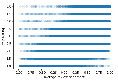
From the previous correlation analysis, we determined that the three features with the strongest correlations to Yelp rating ( the stars column) are average_review_sentiment, average_review_length, and average_review_age.
Let’s better visualize these three features by creating three separate scatterplots where we plot our Yelp rating, stars against average_review_sentiment, average_review_length, and average_review_age, respectively.
# plot stars against average_review_sentiment here
plt.scatter(df['average_review_sentiment'],df['stars'],alpha=0.1)
plt.xlabel('average_review_sentiment')
plt.ylabel('Yelp Rating')
plt.show()
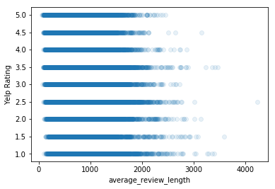
# plot stars against average_review_length here
plt.scatter(df['average_review_length'],df['stars'],alpha=0.1)
plt.xlabel('average_review_length')
plt.ylabel('Yelp Rating')
plt.show()
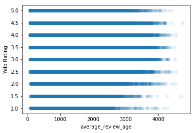
# plot stars against average_review_age against stars here
plt.scatter(df['average_review_age'],df['stars'],alpha=0.1)
plt.xlabel('average_review_age')
plt.ylabel('Yelp Rating')
plt.show()
3.3 Data Selection
Again, the three features with the strongest correlations to Yelp rating are average_review_sentiment, average_review_length, and average_review_age.
Let’s use this knowledge to create our first model with average_review_sentiment, average_review_length, and average_review_age as features.
features = df[['average_review_sentiment','average_review_length','average_review_age']]
ratings = df['stars']
3.4 Split the Data into Training and Testing Sets
Before we can create a model, our data must be separated into a training set and a test set.
X_train, X_test, y_train, y_test = train_test_split(features, ratings, test_size = 0.2, random_state = 1)
3.5 Create and Train the Model
First we need to import LinearRegression from scikit-learn’s linear_model module.
In order to train our model, we will create an instance of the LinearRegression Class, and then use the .fit() method on this instance.
model = LinearRegression()
model.fit(X_train,y_train)
LinearRegression(copy_X=True, fit_intercept=True, n_jobs=None,
         normalize=False)
3.6 Evaluate Model
The effectiveness of our model can be determined with the .score() method, which provides the R^2 value for our model. R^2 values range from 0 to 1, with 0 indicating that 0% of the variability in y can be explained by x, and with 1 indicating the 100% of the variability in y can be explained by x. Let’s use the .score() method on our training and testing sets.
model.score(X_train,y_train)
0.6520510292564032
model.score(X_test,y_test)
0.6495675480094902
We can use .coef_ to generate an array of the feature coefficients determined by fitting our model to the training data. Let’s list the feature coefficients in descending order.
sorted(list(zip(['average_review_sentiment','average_review_length','average_review_age'],model.coef_)),key = lambda x: abs(x[1]),reverse=True)
[('average_review_sentiment', 2.243030310441708),
 ('average_review_length', -0.0005978300178804348),
 ('average_review_age', -0.00015209936823152394)]
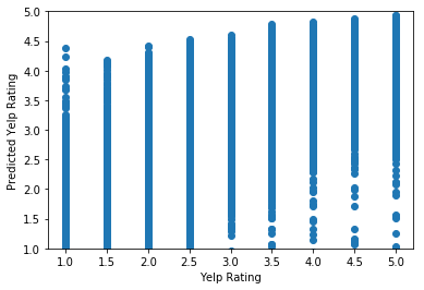
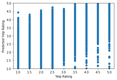
3.7 Data Visualization Pt 2: Scatterplot Predictions
Another way to determine the reliability of the model is to calculate the predicted Yelp ratings for our testing data and compare them to their actual Yelp ratings. We will use a scatterplot to plot Predicted Yelp Rating against the actual Yelp Rating.
We can use the .predict() method to use model’s coefficients to calculate the predicted Yelp rating.
y_predicted = model.predict(X_test)
plt.scatter(y_test,y_predicted)
plt.xlabel('Yelp Rating')
plt.ylabel('Predicted Yelp Rating')
plt.ylim(1,5)
plt.show()
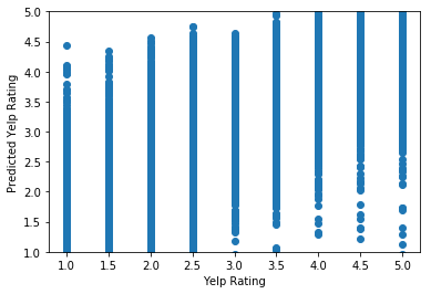
3.8 Future Modeling
Let’s explore the previous process with a new set of features. Instead of re-doing this entire process every time we’d like to change our list of features, we can create a function instead:
# take a list of features to model as a parameter
def model_these_features(feature_list):

    # define ratings and features, with the features limited to our chosen subset of data
    ratings = df.loc[:,'stars']
    features = df.loc[:,feature_list]

    # perform train, test, split on the data
    X_train, X_test, y_train, y_test = train_test_split(features, ratings, test_size = 0.2, random_state = 1)

    # if only one feature is modeled, reshape data to prevent errors
    if len(X_train.shape) < 2:
        X_train = np.array(X_train).reshape(-1,1)
        X_test = np.array(X_test).reshape(-1,1)

    # create and fit the model to the training data
    model = LinearRegression()
    model.fit(X_train,y_train)

    # print the train and test scores
    print('Train Score:', model.score(X_train,y_train))
    print('Test Score:', model.score(X_test,y_test))

    # print the model features and their corresponding coefficients, from most predictive to least predictive
    print(sorted(list(zip(feature_list,model.coef_)),key = lambda x: abs(x[1]),reverse=True))

    # calculate the predicted Yelp ratings from the test data
    y_predicted = model.predict(X_test)

    # plot the actual Yelp Ratings vs the predicted Yelp ratings for the test data
    plt.scatter(y_test,y_predicted)
    plt.xlabel('Yelp Rating')
    plt.ylabel('Predicted Yelp Rating')
    plt.ylim(1,5)
    plt.show()
Let’s use this function on a new set of features.
# subset of all features that have a response range [0,1]
binary_features = ['alcohol?','has_bike_parking','takes_credit_cards','good_for_kids','take_reservations','has_wifi']

# create a model on all binary features here
model_these_features(binary_features)
Train Score: 0.012223180709591164
Test Score: 0.010119542202269072
[('has_bike_parking', 0.19003008208039676), ('alcohol?', -0.14549670708138332), ('has_wifi', -0.13187397577762547), ('good_for_kids', -0.08632485990337231), ('takes_credit_cards', 0.07175536492195614), ('take_reservations', 0.04526558530451594)]

# subset of all features that vary on a greater range than [0,1]
numeric_features = ['review_count','price_range','average_caption_length','number_pics','average_review_age','average_review_length','average_review_sentiment','number_funny_votes','number_cool_votes','number_useful_votes','average_tip_length','number_tips','average_number_friends','average_days_on_yelp','average_number_fans','average_review_count','average_number_years_elite','weekday_checkins','weekend_checkins']

# create a model on all numeric features here
model_these_features(numeric_features)
Train Score: 0.673499259376666
Test Score: 0.6713318798120138
[('average_review_sentiment', 2.2721076642097686), ('price_range', -0.0804608096270259), ('average_number_years_elite', -0.07190366288054195), ('average_caption_length', -0.00334706600778316), ('number_pics', -0.0029565028128950613), ('number_tips', -0.0015953050789039144), ('number_cool_votes', 0.0011468839227082779), ('average_number_fans', 0.0010510602097444858), ('average_review_length', -0.0005813655692094847), ('average_tip_length', -0.0005322032063458541), ('number_useful_votes', -0.00023203784758702592), ('average_review_count', -0.00022431702895061526), ('average_review_age', -0.0001693060816507226), ('average_days_on_yelp', 0.00012878025876700503), ('weekday_checkins', 5.918580754475574e-05), ('weekend_checkins', -5.518176206986478e-05), ('average_number_friends', 4.826992111594799e-05), ('review_count', -3.48348376378989e-05), ('number_funny_votes', -7.884395674183897e-06)]
# all features
all_features = binary_features + numeric_features

# create a model on all features here
model_these_features(all_features)
Train Score: 0.6807828861895333
Test Score: 0.6782129045869245
[('average_review_sentiment', 2.280845699662378), ('alcohol?', -0.14991498593470778), ('has_wifi', -0.12155382629262777), ('good_for_kids', -0.11807814422012647), ('price_range', -0.06486730150041178), ('average_number_years_elite', -0.0627893971389538), ('has_bike_parking', 0.027296969912285574), ('takes_credit_cards', 0.02445183785362615), ('take_reservations', 0.014134559172970311), ('number_pics', -0.0013133612300815713), ('average_number_fans', 0.0010267986822657448), ('number_cool_votes', 0.000972372273441118), ('number_tips', -0.0008546563320877247), ('average_caption_length', -0.0006472749798191067), ('average_review_length', -0.0005896257920272376), ('average_tip_length', -0.00042052175034057535), ('number_useful_votes', -0.00027150641256160215), ('average_review_count', -0.00023398356902509327), ('average_review_age', -0.00015776544111326904), ('average_days_on_yelp', 0.00012326147662885747), ('review_count', 0.00010112259377384992), ('weekend_checkins', -9.239617469645031e-05), ('weekday_checkins', 6.1539091231461e-05), ('number_funny_votes', 4.8479351025072536e-05), ('average_number_friends', 2.0695840373717654e-05)]
3.9 Prediction of a Hypothetical Restaurant: Adrian’s Taco Shop
Let’s create a hypothetical restaurant and predict its Yelp Rating. First, let’s recall what our features are.
print(all_features)
['alcohol?', 'has_bike_parking', 'takes_credit_cards', 'good_for_kids', 'take_reservations', 'has_wifi', 'review_count', 'price_range', 'average_caption_length', 'number_pics', 'average_review_age', 'average_review_length', 'average_review_sentiment', 'number_funny_votes', 'number_cool_votes', 'number_useful_votes', 'average_tip_length', 'number_tips', 'average_number_friends', 'average_days_on_yelp', 'average_number_fans', 'average_review_count', 'average_number_years_elite', 'weekday_checkins', 'weekend_checkins']
For some perspective on preexisting restaurants, let’s calculate the mean, minimum, and maximum values for each feature.
pd.DataFrame(list(zip(features.columns,features.describe().loc['mean'],features.describe().loc['min'],features.describe().loc['max'])),columns=['Feature','Mean','Min','Max'])
| Feature | Mean | Min | Max | |
|---|---|---|---|---|
| 0 | average_review_sentiment | 0.554935 | -0.995200 | 0.996575 |
| 1 | average_review_length | 596.463567 | 62.400000 | 4229.000000 |
| 2 | average_review_age | 1175.501021 | 71.555556 | 4727.333333 |
Let’s call our hypothetical restaurant Adrian's Taco Shop and assign this taco shop reasonable values for each feature.
adrians_taco_shop = np.array([1,1,1,1,1,1,75,2,3,10,10,1200,0.95,3,6,10,50,3,50,500,20,100,1,0,0]).reshape(1,-1)
Before we make a prediction, let’s retrain our model on all our features.
#retrain model on all features
features = df.loc[:,all_features]
ratings = df.loc[:,'stars']
X_train, X_test, y_train, y_test = train_test_split(features, ratings, test_size = 0.2, random_state = 1)
model = LinearRegression()
model.fit(X_train,y_train)
LinearRegression(copy_X=True, fit_intercept=True, n_jobs=None,
         normalize=False)
Finally, let’s make our Yelp rating prediction on Adrian's Taco Shop!
model.predict(adrians_taco_shop)
array([3.82929417])
3.8 stars, huh……. Not too bad, I guess.
4 Discussion & Conclusion
We were able to build a Multiple Linear Regression model with the capability to somewhat predict a restaurant’s Yelp rating. Although we obtained our highest Test Score of 0.6713318798120138 when modeling all available features, this test score was not much higher than when we modeled only numeric features or our top 3 features.
This project demonstrated that even if a plethora of data is available, it can still be difficult to make predictions. Additonally, I learned how initial analysis can provide valuable insight for future projects.
For example, we determined that average_review_sentiment has the strongest correlation with Yelp rating; it might be worth further investigating how “sentiment” is determined by using Natural Language Processing techniques. (More on NLP soon!)