Visualization of Perceptron Logic Gates

1 Introduction

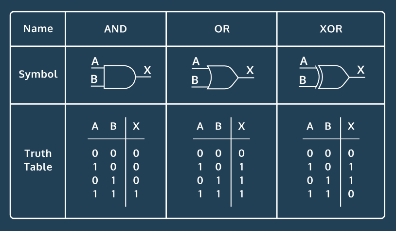
I will use perceptrons to model the fundamental building blocks of computers — logic gates. This project will focus on AND, OR, and XOR Logic Gates and use the data from their respective truth tables.

1.1 Goal:

• Demonstrate how a perceptron model can be used as a linear classifier tool

1.2 Approach:

• Visualize the respective decision boundary of each logic gate
  • Demonstrate how AND, OR gates can represent linearly separable data
  • Demonstrate how a XOR gate can represent non-linearly-separable data

1.3 Imports

Import libraries and write settings here.

# Data manipulation
import numpy as np
from itertools import product

# Machine Learning
from sklearn.linear_model import Perceptron

# Visualizations
%matplotlib inline
import matplotlib.pyplot as plt

2 Analysis/Modeling

2.0.1 Create Data Points

First, let’s look at the A and B columns of our truth table. We can think of each column as a single input, and we can combine these two inputs to create a set of four points.

#list of four possible inputs to gate
data = [[0,0], [0,1], [1,0], [1,1]]

2.0.2 Create Labels

We will find the labels for our AND, OR, and XOR logic gates under its corresponding X column in the truth table. Let’s create a list of labels for each gate.

#AND, OR, and XOR gate labels
ANDlabels = [0, 0, 0, 1]
ORlabels = [0, 1, 1, 1]
XORlabels = [0, 1, 1, 0]

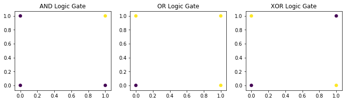
2.0.3 Data Visualization Pt. 1: Labeled Scatterplots

Before can create a scatterplot, we need to break down our data into its x and y values. We can do this with a list comprehension. Then, we can plot our x_values and y_values on three different scatterplots, colorizing differences between the three gates.

#generate x and y values from data
x_values = [point[0] for point in data]
y_values = [point[1] for point in data]

#plot AND gate
fig = plt.figure(figsize = (12,3))
plt.subplot(1,3,1)
plt.scatter(x_values, y_values, c=ANDlabels)
plt.title("AND Logic Gate")

#plot OR gate
plt.subplot(1,3,2)
plt.scatter(x_values, y_values, c=ORlabels)
plt.title("OR Logic Gate")

#plot XOR gate
plt.subplot(1,3,3)
plt.scatter(x_values, y_values, c=XORlabels)
plt.title("XOR Logic Gate")
plt.show()

2.0.4 Results & Discussion

Each scatterplot displays 4 points, and each point represents a specific color.

In the context of these scatterplots, we can think of a “decision boundary” as a “straight line separating the two colors.” In other words, if a straight line can be drawn across a scatterplot where only a single color remains on either side of the line, then we can conclude that the data is linearly separable.

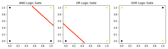
The drawn red line is an estimation of where the decision boundary should be located.

A line can be successfully drawn on the AND, OR graphs indicating that these logic gates are linearly separable. This line cannot be drawn on the XOR graph, indicating that the XOR logic gate is not linearly separable.

2.1.0 Create the Perceptron Model

Using our data and labels, let’s build a perceptron to learn AND, OR, and XOR.

#create perceptron object
classifier = Perceptron(max_iter=40, tol=1e-3)

2.1.1 Train and Evaluate Model

Normally, we wouldn’t train and test our model on the same dataset. However, in our scenario there are only four possible inputs to each gate, so we’re stuck training on every possible input and testing on those same points.

We can use the .score() method to print the accuracy of the model on the data points.

#train model, and print accuracy of model on the data points
classifier.fit(data, ANDlabels)
print(classifier.score(data, ANDlabels))
#output of 1.0 indicates that 100% of the time, model was able to correctly determine output given data

classifier.fit(data, ORlabels)
print(classifier.score(data, ORlabels))
#output of 1.0 indicates that 100% of the time, model was able to correctly determine output given data

classifier.fit(data, XORlabels)
print(classifier.score(data, XORlabels))
#output of 0.5 indicates that 50% of the time, model was able to correctly determine output given data

1.0
1.0
0.5

2.1.2 Results & Discussion

The AND & OR logic gates both had an output score of 1.0 which indicates that 100% of the time the model was able to correctly determine output given data. Thus, these two gates are linearly seperable; in other words, a decision boundary exists.

The XOR logic gates had an output score of 0.5 which indicates that only 50% of the time the model was able to correctly determine output given data. Thus, XOR is not linearly seperable; in other words, a decision boundary does not exist.

2.2.0 The Decision Function

We can use the .decision_function method to calculate the distance between a particular point and the decision boundary of a dataset. For example:

#decision function can tell us the proximity of a particular point from the decision boundary
#example:
print(classifier.decision_function([[0, 0], [1, 1], [0.5, 0.5]]))

[ 0.  -1.  -0.5]

In this example, decision_function tells us that points [0, 0], [1, 1], [0.5, 0.5] are 0, -1.0, and -0.5 units away from XOR decision boundary.

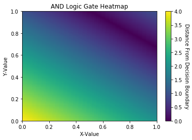
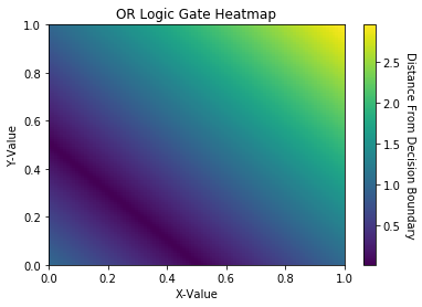
2.3.0 Data Visualization Pt. 2: Decision Boundary Heatmaps

Let’s use the capability of the decision_function to create a heatmap for each logic gate. Each heatmap will contain 100 equidistant, ordered pairs and their respective distances from the decision boundary.

#create 100 equidistant, ordered pairs
x_values = np.linspace(0, 1, 100)
y_values = np.linspace(0, 1, 100)
point_grid = list(product(x_values, y_values))

#plot heatmap for AND gate
classifier.fit(data, ANDlabels)
distances = classifier.decision_function(point_grid)
abs_distances = [abs(pt) for pt in distances]
distances_matrix = np.reshape(abs_distances, (100,100))

heatmap = plt.pcolormesh(x_values, y_values, distances_matrix)
cbar = plt.colorbar(heatmap)
plt.xlabel("X-Value")
plt.ylabel("Y-Value")
plt.title("AND Logic Gate Heatmap")
cbar.set_label("Distance From Decision Boundary", rotation=270, labelpad=13)
plt.show()

#plot heatmap for OR gate
classifier.fit(data, ORlabels)
distances = classifier.decision_function(point_grid)
abs_distances = [abs(pt) for pt in distances]
distances_matrix = np.reshape(abs_distances, (100,100))

heatmap = plt.pcolormesh(x_values, y_values, distances_matrix)
cbar = plt.colorbar(heatmap)
plt.xlabel("X-Value")
plt.ylabel("Y-Value")
plt.title("OR Logic Gate Heatmap")
cbar.set_label("Distance From Decision Boundary", rotation=270,labelpad=13)
plt.show()

#plot heatmap for XOR gate
classifier.fit(data, XORlabels)
distances = classifier.decision_function(point_grid)
abs_distances = [abs(pt) for pt in distances]
distances_matrix = np.reshape(abs_distances, (100,100))

heatmap = plt.pcolormesh(x_values, y_values, distances_matrix)
cbar = plt.colorbar(heatmap)
plt.xlabel("X-Value")
plt.ylabel("Y-Value")
plt.title("XOR Logic Gate Heatmap")
cbar.set_label("Distance From Decision Boundary", rotation=270, labelpad=13)
plt.show()

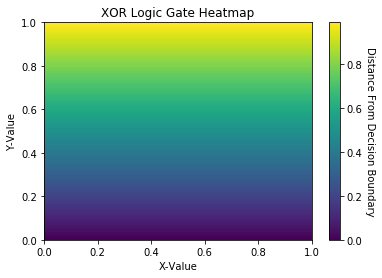
2.3.1 Results & Discussion

The deep purple region of the AND & OR logic gate heatmap represents its respective decision boundary. In the XOR heatmap, the deep purple region is unable to seperate data into 2 distinct regions. Thus, the XOR heatmap illustrates data that is not linearly seperable.

3 Conclusions and Next Steps

A single perceptron with only two inputs can only solve problems that are linearly seperable because it cannot represent a non-linear decision boundary.

However, by increasing the number of features and perceptrons, we can give rise to the Multilayer Perceptrons, also known as Neural Networks, which can solve much more complicated problems. More on Neural Networks in future posts! :-)