Breast Cancer Classifier

1 Introduction

Typically, to determine whether a tumor is benign or cancerous, a doctor will take sample of the cells with a biopsy procedure and consequently send this sample to a pathologist for analysis. Although this approach is effective for classifying tumors, feedback is not immediate; this could prove harmful if the prognosis is time sensitive.

This project will demonstrate how algorithms can be utilized to provide accurate, immediate feedback for time sensitive medical issues.

1.1 Goal

• Demonstrate how a K-Nearest Neighbors model can be used to classify a patient’s breast mass as malignant or benign

1.2 Approach

• Perform statistical analysis on the UCI ML Breast Cancer Wisconsin (Diagnostic) Data Set

1.3 Imports

# UCI ML Breast Cancer Wisconsin (Diagnostic) Data Set
from sklearn.datasets import load_breast_cancer

# Machine Learning
from sklearn.model_selection import train_test_split
from sklearn.neighbors import KNeighborsClassifier

# Visualizations
%matplotlib inline
import matplotlib.pyplot as plt

2 Explore Data

2.1 Explore Features

In the cell above, we imported the UCI ML Breast Cancer Wisconsin (Diagnostic) Data Set. Let’s load this data into a variable breast_cancer_data and then print all of our data’s features.

# load UCI ML Breast Cancer Wisconsin (Diagnostic) Data Set
breast_cancer_data = load_breast_cancer()

# print all features
print(breast_cancer_data.feature_names)

['mean radius' 'mean texture' 'mean perimeter' 'mean area'
 'mean smoothness' 'mean compactness' 'mean concavity'
 'mean concave points' 'mean symmetry' 'mean fractal dimension'
 'radius error' 'texture error' 'perimeter error' 'area error'
 'smoothness error' 'compactness error' 'concavity error'
 'concave points error' 'symmetry error' 'fractal dimension error'
 'worst radius' 'worst texture' 'worst perimeter' 'worst area'
 'worst smoothness' 'worst compactness' 'worst concavity'
 'worst concave points' 'worst symmetry' 'worst fractal dimension']

Next, let’s print our first datapoint. Each number in the output corresponds to its respective feature.

# print first datapoint
print(breast_cancer_data.data[0])

[1.799e+01 1.038e+01 1.228e+02 1.001e+03 1.184e-01 2.776e-01 3.001e-01
 1.471e-01 2.419e-01 7.871e-02 1.095e+00 9.053e-01 8.589e+00 1.534e+02
 6.399e-03 4.904e-02 5.373e-02 1.587e-02 3.003e-02 6.193e-03 2.538e+01
 1.733e+01 1.846e+02 2.019e+03 1.622e-01 6.656e-01 7.119e-01 2.654e-01
 4.601e-01 1.189e-01]

2.2 Explore Labels

We can find the labels associated with every data point by using breast_cancer_data.target. In this case, our labels are either 0 or 1 and refer to malignant or benign, respectively

# print target label values
print(breast_cancer_data.target)

[0 0 0 0 0 0 0 0 0 0 0 0 0 0 0 0 0 0 0 1 1 1 0 0 0 0 0 0 0 0 0 0 0 0 0 0 0
 1 0 0 0 0 0 0 0 0 1 0 1 1 1 1 1 0 0 1 0 0 1 1 1 1 0 1 0 0 1 1 1 1 0 1 0 0
 1 0 1 0 0 1 1 1 0 0 1 0 0 0 1 1 1 0 1 1 0 0 1 1 1 0 0 1 1 1 1 0 1 1 0 1 1
 1 1 1 1 1 1 0 0 0 1 0 0 1 1 1 0 0 1 0 1 0 0 1 0 0 1 1 0 1 1 0 1 1 1 1 0 1
 1 1 1 1 1 1 1 1 0 1 1 1 1 0 0 1 0 1 1 0 0 1 1 0 0 1 1 1 1 0 1 1 0 0 0 1 0
 1 0 1 1 1 0 1 1 0 0 1 0 0 0 0 1 0 0 0 1 0 1 0 1 1 0 1 0 0 0 0 1 1 0 0 1 1
 1 0 1 1 1 1 1 0 0 1 1 0 1 1 0 0 1 0 1 1 1 1 0 1 1 1 1 1 0 1 0 0 0 0 0 0 0
 0 0 0 0 0 0 0 1 1 1 1 1 1 0 1 0 1 1 0 1 1 0 1 0 0 1 1 1 1 1 1 1 1 1 1 1 1
 1 0 1 1 0 1 0 1 1 1 1 1 1 1 1 1 1 1 1 1 1 0 1 1 1 0 1 0 1 1 1 1 0 0 0 1 1
 1 1 0 1 0 1 0 1 1 1 0 1 1 1 1 1 1 1 0 0 0 1 1 1 1 1 1 1 1 1 1 1 0 0 1 0 0
 0 1 0 0 1 1 1 1 1 0 1 1 1 1 1 0 1 1 1 0 1 1 0 0 1 1 1 1 1 1 0 1 1 1 1 1 1
 1 0 1 1 1 1 1 0 1 1 0 1 1 1 1 1 1 1 1 1 1 1 1 0 1 0 0 1 0 1 1 1 1 1 0 1 1
 0 1 0 1 1 0 1 0 1 1 1 1 1 1 1 1 0 0 1 1 1 1 1 1 0 1 1 1 1 1 1 1 1 1 1 0 1
 1 1 1 1 1 1 0 1 0 1 1 0 1 1 1 1 1 0 0 1 0 1 0 1 1 1 1 1 0 1 1 0 1 0 1 0 0
 1 1 1 0 1 1 1 1 1 1 1 1 1 1 1 0 1 0 0 1 1 1 1 1 1 1 1 1 1 1 1 1 1 1 1 1 1
 1 1 1 1 1 1 1 0 0 0 0 0 0 1]

# print target label names, in this case 'benign' or 'malignant'
print(breast_cancer_data.target_names)

['malignant' 'benign']

3 Exploratory Analysis

3.1 Split the Data into Training and Testing Sets

Before we can create a model, our data must be separated into a training set and a test set. Deciding how to split our data into training and testing sets is a tricky question.

If the training set is too small, then the algorithm might not have enough data to effectively learn. However, if the training set is too big, then the algorithm will overfit the training model, rendering the model unable to effectively generalize.

A general rule of thumb is to put 80% of your data in the training set and around 20% of your data and the validation set. In this project, we will follow the rule of thumb.

# prepare training set, validation set, training labels, validation labels
training_data, validation_data, training_labels, validation_labels = train_test_split(
        breast_cancer_data.data,
        breast_cancer_data.target,
        test_size=0.2,
        random_state=100
)

3.2 Create and Train the Model

We previously imported KNeighborsClassifier from scikit-learn’s neighbors module.

In order to train our model, we will create an instance of the KNeighborsClassifier Class, and then use the .fit() method on this instance. For this preliminary model, we will set k = 3.

# create instance of KNeighborsClassifier
classifier = KNeighborsClassifier(n_neighbors = 3)

# train classifier
classifier.fit(training_data, training_labels)

KNeighborsClassifier(algorithm='auto', leaf_size=30, metric='minkowski',
           metric_params=None, n_jobs=None, n_neighbors=3, p=2,
           weights='uniform')

3.3 Evaluate Model

We can use the .score method to evaluate how accurately the model can classify a tumor as malignant or benign.

print(classifier.score(validation_data, validation_labels))

0.9473684210526315

Our model was able to correctly classify a tumor ~94% of the time! Let’s see if we can improve our model’s accuracy…

3.4 Model Modifications Pt. 1: K-Value

One fundamental question when building a K-Nearest Neighbors model is: “Which K Value should I use?”

Instead of guessing random values, let’s investigate how changing our k-value affects model accuracy by using a for loop!

# iterate model 100 times using k-values 1 to 100
accuracies = []
for k in range(1, 101):
    classifier = KNeighborsClassifier(n_neighbors=k)
    classifier.fit(training_data, training_labels)
    accuracies.append(classifier.score(validation_data, validation_labels))

print(accuracies)

[0.9298245614035088, 0.9385964912280702, 0.9473684210526315, 0.9473684210526315, 0.9473684210526315, 0.9473684210526315, 0.9473684210526315, 0.9473684210526315, 0.956140350877193, 0.956140350877193, 0.956140350877193, 0.956140350877193, 0.956140350877193, 0.956140350877193, 0.956140350877193, 0.956140350877193, 0.956140350877193, 0.956140350877193, 0.956140350877193, 0.956140350877193, 0.956140350877193, 0.956140350877193, 0.9649122807017544, 0.9649122807017544, 0.956140350877193, 0.956140350877193, 0.956140350877193, 0.956140350877193, 0.9473684210526315, 0.9473684210526315, 0.9473684210526315, 0.9473684210526315, 0.9473684210526315, 0.9473684210526315, 0.9473684210526315, 0.9473684210526315, 0.956140350877193, 0.956140350877193, 0.956140350877193, 0.956140350877193, 0.956140350877193, 0.956140350877193, 0.956140350877193, 0.9473684210526315, 0.956140350877193, 0.9473684210526315, 0.956140350877193, 0.956140350877193, 0.956140350877193, 0.956140350877193, 0.9473684210526315, 0.9473684210526315, 0.9473684210526315, 0.956140350877193, 0.956140350877193, 0.9649122807017544, 0.9473684210526315, 0.9473684210526315, 0.9385964912280702, 0.9298245614035088, 0.9298245614035088, 0.9385964912280702, 0.9473684210526315, 0.9385964912280702, 0.9385964912280702, 0.9385964912280702, 0.9385964912280702, 0.9385964912280702, 0.9385964912280702, 0.9385964912280702, 0.9385964912280702, 0.9385964912280702, 0.9385964912280702, 0.9385964912280702, 0.9385964912280702, 0.9385964912280702, 0.9298245614035088, 0.9298245614035088, 0.9298245614035088, 0.9298245614035088, 0.9210526315789473, 0.9298245614035088, 0.9210526315789473, 0.9385964912280702, 0.9298245614035088, 0.9385964912280702, 0.9385964912280702, 0.9385964912280702, 0.9298245614035088, 0.9298245614035088, 0.9210526315789473, 0.9385964912280702, 0.9210526315789473, 0.9298245614035088, 0.9298245614035088, 0.9385964912280702, 0.9298245614035088, 0.9385964912280702, 0.9298245614035088, 0.9298245614035088]

We iterated the model 100 times, using the integer values from 1 to 100 as our k values. First, let’s determine the greatest value in our accuracies list. Then, let’s use a list comprehension to find the k-value(s) associated with the highest accuracy.

# print highest accuracy value
print(max(accuracies))

0.9649122807017544

# create list of k-value(s) associated with the highest accuracy
accurate_k = [i for i,x in enumerate(accuracies) if x == max(accuracies)]
print(accurate_k)

[22, 23, 55]

3.5 Data Visualization: Model Accuracy vs K-Value Scatterplot

Before selecting a K-Value, let’s expand on the previous section by plotting the change in model accuracy as its K-Value is adjusted.

# create list of x values from 1 to 100
k_list = range(1, 101)

# create scatterplot displaying accuracies vs k_list
plt.plot(k_list, accuracies)
plt.xlabel('k')
plt.ylabel('Validation Accuracy')
plt.title('Breast Cancer Classifier Accuracy')
plt.show()

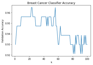
3.6 Selecting a K-Value

By looking at the scatterplot, we can see that model accuracy:

• sharply increases from k changes from 1-10
• sporadically changes within a fixed interval as k changes from 10-55
• sharply decreases as k increases over 55

Also, from the previous section we determined that our most accurate k-values were [22, 23, 55].

When selecting a K-Value for a KNN algorithm, there are a few guidelines that should be considered:

• K value should be odd
  • Immediately, this eliminates 22 as an option
• K value must not be multiples of the number of classes (In our case, there are two classes)
  • Again, this eliminates 22 as an option
• Should not be too small or too large

We are left with 23 and 55 as potential options. When considering that:

• graph results indicate a sharp decrease in accuracy beginning at k = 55
• 55 is a relatively large number in the context of this model

I believe that we should use a k-value of 23.

3.7 Model Modifications Pt. 2: Random State

The random state is an arbitrary number that will change which points are in the training set and which are in the validation set. Originally, we used a random state of 100.

# prepare training set, validation set, training labels, validation labels
training_data, validation_data, training_labels, validation_labels = train_test_split(
        breast_cancer_data.data,
        breast_cancer_data.target,
        test_size=0.2,
        random_state=100
)

# create instance of KNeighborsClassifier
classifier = KNeighborsClassifier(n_neighbors = 23)

# train classifier
classifier.fit(training_data, training_labels)

# print model accuracy
print(classifier.score(validation_data, validation_labels))

0.9649122807017544

Let’s create two different versions of our model: one where we decrease random_state and one where we increase random_state.

# prepare training set, validation set, training labels, validation labels
training_data, validation_data, training_labels, validation_labels = train_test_split(
        breast_cancer_data.data,
        breast_cancer_data.target,
        test_size=0.2,
        random_state=80
)

# create instance of KNeighborsClassifier
classifier = KNeighborsClassifier(n_neighbors = 23)

# train classifier
classifier.fit(training_data, training_labels)

# print model accuracy
print(classifier.score(validation_data, validation_labels))

0.9385964912280702

# prepare training set, validation set, training labels, validation labels
training_data, validation_data, training_labels, validation_labels = train_test_split(
        breast_cancer_data.data,
        breast_cancer_data.target,
        test_size=0.20,
        random_state=120
)

# create instance of KNeighborsClassifier
classifier = KNeighborsClassifier(n_neighbors = 23)

# train classifier
classifier.fit(training_data, training_labels)

# print model accuracy
print(classifier.score(validation_data, validation_labels))

0.9385964912280702

After modifying the random_state of each model, scores of 0.9385964912280702 and 0.9385964912280702 were obtained. Both of these score are lower than the original value. There is no compelling reason to adjust the model’s original random_state of 100.

4 Discussion & Conclusion

By using a K-value of 23 and a random_state of 100, we were able to build a K-Nearest Neighbors model with the capability to correctly classify a patient’s breast mass ~96.4% of the time!

In this project, I learned that lingering on small details can hamper progress. In most cases, it can be more useful to simply devise a preliminary model and then make adjustments as needed. Additionally, unless there is convincing evidence, model parameters should not be changed simply for the sake of “changing parameters”.

More importantly, this project is an example of how big data analytics can potentially challenge our traditional, reactive healthcare system and, instead, instate a predictive, proactive, and preventative approach. K-Nearest Neighbors is only one of various algorithms that can be applied to cancer diagnosis research. For instance, clinical imaging data can be used in conjunction with computer vision tools to detect cancer. More on computer vision in future posts! :)